Lab 1 is meant to assess students knowledge of geographic and projected coordinate systems. Students should be able to define and project data to be usable for GIS analysis. Two maps will be generated through this lab. The first will be a comparison map of seven coordinate systems. The second will be a map of rivers in central Wisconsin meant to showcase the students ability to correct missing spatial references.
Methods
A geographic coordinate system (GCS) uses a 3-dimensional spherical surface to locate features on the earths surface, commonly denoted with Latitude and Longitude. Using a GCS will result in distortions of one or more of the following: area, length, and angle.
A projected coordinate system (PCS) uses a 2-dimensional flat surface to locate feature on the earths surface. A PCS will show a target area without distortion but only for that specific area. The farther away from the target area, the greater the distortion.
Projected coordinate systems are based on Geographic coordinate systems. A GCS is needed to map a feature or area and a PCS refines the map to allow for accurate measurements and visualizations.
ArcMap 10.2 will be used to create the two maps needed for this lab. To illustrate what went into creating these maps, some basics of ArcMap will be described along with a short example walkthrough and different Tool descriptions.
- ArcMap Basics -
Figure 1: This is a Blank Map in ArcMap 10.2.

Figure 2: The Catalog window allows for quick and easy management of files. Click, drag, and drop a file into the workspace to add data to the map.

Figure 3: The Table of Contents contains each data layer and it's associated data. Shape files and other data can be rearranged and modified from this window. What is seen in the Table of Contents is only a reference to the actual data, not the data itself. Therefore, any changes that are made are not permanent.

Figure 4: The Data Frame Properties is accessed by right clicking the Layers heading in the Table of Contents. Here general information for the data frame is displayed and different settings can be changed and modified for the entire data frame. Changing the coordinate system in the Data Frame Properties will only change how the data is displayed for that specific data frame, it will not change the individual files coordinate systems.

Figure 5: The Layer Properties window is accessed by right clicking a layer name in the Table of Contents. Here general information for the data in the layer is displayed and different settings can be changed and modified for that specific layer.


Figure 6: To add a data frame (picture on the left), click Insert on the main toolbar and choose Data Frame. The resulting New Data Frame (picture on the right) will appear underneath any data frames already created and will automatically be set as active.
- Example walk through -
(importing data, selections, creating shapefiles)

Figure 7: The shape file states.shp was added to the workspace from the Catalog window. The data can now be modified and utilized in ArcMap.

Figure 8: To make a selection, click Selection on the main toolbar and choose either Select By Attributes or Select By Location. Here, Wisconsin will be selected by choosing Select By Attributes.

Figure 9: The Attribute Table contains all the data associated with a file. It can be accessed by right clicking a layer in the Table of Contents. Here information can be gathered to fully utilize the Select by Attributes option.

Figure 10: After clicking the Select by Attributes option, the Select of Attributes window will appear. Using the fields available and typing with the keyboard, the phrase, State_Name = 'Wisconsin', is entered into the bottom of the window (use single quotations when selecting text). Once Apply or Ok is clicked, the state of Wisconsin is selected in light blue.

Figure 11: Now that Wisconsin is selected it can be made into its own layer. Right click the layer the selection is referencing, hovering over Selection, then clicking Create Layer From Selected Features. This will create a separate layer with just Wisconsin.

Figure 12: The new Wisconsin layer is shown in a different color and placed above the layer that was used to make the selection.

Figure 13: Now the layer can be exported as its own shapefile. This is done by right clicking the new Wisconsin layer, hovering over Data, and selecting Export Data....

Figure 14: After clicking Export Data..., the Export Data window appears. Here the location of the new feature class is designated. When saving, the option for Save as type should be set to Shapefile.

Figure 15: The resulting shapefile.
- Tools for Projections -
(Define Projection and Project)


Figure 16: The ArcToolbox (expanded on the left to show the location of projection tools used in this lab). The ArcToolbox can be accessed by clicking the toolbox icon on the main toolbar or can be found in the Catalog Window.

Figure 17: Clicking Define Projection from the toolbox will result in the Define Projection Window. From this window, the feature class that needs defining is chosen along with its newly defined coordinate system. The Define Projection tool is used for feature classes that are missing spatial references. After the tool is run the feature class is now labeled correctly.

Figure 18: Clicking Project from the toolbox will result in the Project Window. From this window, the feature class that needs projection along with the desired new coordinate system can be chosen. The Project tool is used to change the coordinate system for a layer. Unlike changing the coordinate system for the data frame, this change is permanent.
Results
Using the skills and tools described above, these two maps were created.

Figure 19: Map comparing 7 different coordinate systems. The top most displays a geographic coordinate system, while the rest depict varying projected coordinate systems.
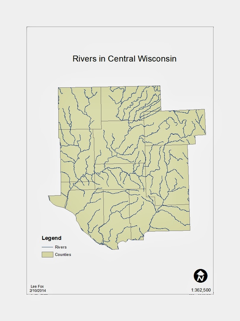
Figure 20: Map displaying the rivers of central Wisconsin along with a portion of Wisconsin. Both these files had projection abnormalities that were corrected by using both the Define Projection tool and the Project tool.