Lab 3: Multiple Criteria Query

Introduction

 This lab is meant to test students knowledge of attribute and spatial queries. Students will need to write multiple criteria queries to extract specific information from a database. Each query should be written as concisely as possible and return the correct information.


Methods

Boolean operators are used to create logical expressions that relate data together through satisfying combinations of conditions. For this lab, the Boolean operators AND, OR, and IN are used.

 AND - returns records that satisfies both conditions

Figure 1: In this diagram the red section symbolizes the records that satisfy the conditions. A and B symbolize different data sets.

 OR - returns records that satisfies either condition

 Figure 2: In this diagram the red section symbolizes the records that satisfy the conditions. A and B symbolize different data sets. 

IN - returns records that have one of several strings or values inside the parenthesis

EXAMPLE:              "STATE_NAME" IN ('Wisconsin', 'Minnesota')

In this example, all records from Wisconsin or Minnesota will be returned, but none from any other state.

Figure 3: Select by Attributes. The red area indicates the drop down menu to select the layer to use. The blue area indicates the drop down menu to select the selection method, either "Create a new selection" or " Select from current selection." The yellow area lists the fields of the data set and is also where the fields of interest can be chosen when constructing the query. The green area is where the query is entered through a combination of choosing fields from the yellow area, choosing the operators underneath the yellow area, and using the keyboard. For this lab, this green area is where the Boolean expressions are made.

Results

 - First Map -

- Second Map -

 - Third Map -

 - Fourth Map -

 

- Fifth Map -

 

 

Lab 2: Downloading and Mapping GIS Data

Introduction

This lab is meant to give students hands-on experience in utilizing on-line resources for data collection, specifically the US Census Bureau's website, and manipulating the data to be useful in GIS analysis. Completing this lab will showcase the students ability to download tabular data and shape files from the US Census Bureau's website, join standalone tables to attribute tables, create appropriate maps, and build visually pleasing layouts. Two maps will be generate through this lab. The first will be a population density map of Wisconsin and the second will display any chosen variable available to the student, downloaded from the US Census Bureau's website, concerning Wisconsin.

The US Census Bureau's mission is "To serve as the leading source of quality data about the nation's people and economy." They do this by attempting "To provide the best mix of timeliness, relevancy, quality, and cost for the data we collect and services we provide." Different data is collected at different time intervals; a population and housing census is done every 10 years, an economic census and government census is done every 5 years, and as of 2010 the American Community Survey is done annually. To learn more about the US Census visit their website here: About Us

The data that will be downloaded and utilized for this lab is "2010 SF1 100% Data" which is collected every 10 years. This data is the most basic of all census data and includes: total population, age cohorts, household size, racial breakdowns, housing units, relationships in households, and renter/owner occupied.

Methods

To begin, navigate to this website: American Fact Finder

Part I - Downloading Data

Figure 1: The American fact finder website. Click advanced search to continue.

Figure 2: The advanced search page. Click Topics to pick the area of interest. Here the data set can be chosen. Clicking the area of interest will place it in the upper left corner of the screen in the "Your Selections" box.

Figure 3: Next click on Geographies. Here the area of interest can be chosen. Clicking Add To Your Selections will place the area of interest in the "Your Selections" box.

Figure 4: Once the Topic and Geographies are chosen, the data set(s) can be chosen by filling in the box next to the name of the desired data set. Then click download.

The data will be downloaded as a .zip file. Extracting the contents will result in two excel tables. One is the metadata and the other is the census data. The census data has a field named GEO#id which will be used to join the data to a shape file that will be downloaded next.

Part II - Downloading Shape Files



Figure 5: In Geographies, click the map tab. This will bring up the shape file for the area of interest. Click the download button to open the Download window.

Figure 6: The Download window. Here options for which type of data should be downloaded are chosen. Shapefiles are at the bottom.

The shape file comes in a .zip format as well and will need to be extracted the same way as the data. The shape file can then be opened in ArcMap.



Figure 7: Here is the shape file displayed in ArcMap without any joins or symbolization. The excel table can also be seen in the Table of Contents.

Figure 8: The attribute tables for both the shape file (right) and the excel table (left) are shown. The GEO#id field in the excel table and the GEO_ID field in the shape file's table will be used as the foundations for a one-to-one cardinality attribute join.

Figure 9: Right click the shape file in the table of contents, hover over Joins and Relates, and click join. This window will appear. Chose the correct fields and table for the join and click OK.

Figure 10: This is the resulting table after the excel spreadsheet was joined to the shape file.

Figure 11: Right click on the shape file in the Table of Contents and select the symbology tab. Click the dropdown menu for Value to add the data to be mapped. Click the dropdown menu for Normalization if the data to be mapped needs it. In this case it does because the variable that is being mapped in population.

Results

 

Figure 12: The final output of the Lab. A map showing population density and a map showing household occupancy for the state of Wisconsin.

Lab 1: Coordinate Systems and Map Projection

Introduction

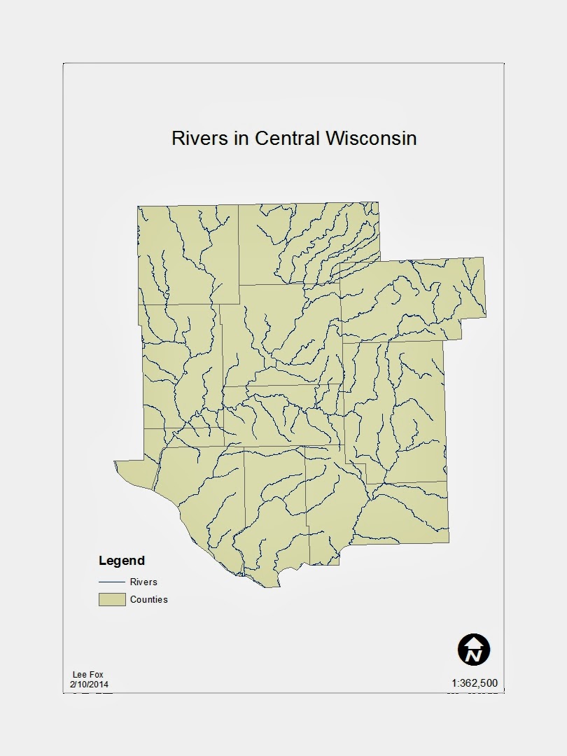
Lab 1 is meant to assess students knowledge of geographic and projected coordinate systems. Students should be able to define and project data to be usable for GIS analysis. Two maps will be generated through this lab. The first will be a comparison map of seven coordinate systems. The second will be a map of rivers in central Wisconsin meant to showcase the students ability to correct missing spatial references.

Methods

A geographic coordinate system (GCS)  uses a 3-dimensional spherical surface to locate features on the earths surface, commonly denoted with Latitude and Longitude. Using a GCS will result in distortions of one or more of the following: area, length, and angle.

A projected coordinate system (PCS) uses a 2-dimensional flat surface to locate feature on the earths surface. A PCS will show a target area without distortion but only for that specific area. The farther away from the target area, the greater the distortion.

Projected coordinate systems are based on Geographic coordinate systems. A GCS is needed to map a feature or area and a PCS refines the map to allow for accurate measurements and visualizations.

ArcMap 10.2 will be used to create the two maps needed for this lab. To illustrate what went into creating these maps, some basics of ArcMap will be described along with a short example walkthrough and different Tool descriptions.

 

- ArcMap Basics -

 



Figure 1: This is a Blank Map in ArcMap 10.2.

 

Figure 2: The Catalog window allows for quick and easy management of files. Click, drag, and drop a file into the workspace to add data to the map.

 

 

 

 Figure 3: The Table of Contents contains each data layer and it's associated data. Shape files and other data can be rearranged and modified from this window. What is seen in the Table of Contents is only a reference to the actual data, not the data itself. Therefore, any changes that are made are not permanent.

 

 

 

Figure 4: The Data Frame Properties is accessed by right clicking the Layers heading in the Table of Contents. Here general information for the data frame is displayed and different settings can be changed and modified for the entire data frame. Changing the coordinate system in the Data Frame Properties will only change how the data is displayed for that specific data frame, it will not change the individual files coordinate systems.

 

 

Figure 5: The Layer Properties window is accessed by right clicking a layer name in the Table of Contents. Here general information for the data in the layer is displayed and different settings can be changed and modified for that specific layer.

 

 

 

 

Figure 6: To add a data frame (picture on the left), click Insert on the main toolbar and choose Data Frame. The resulting New Data Frame (picture on the right) will appear underneath any data frames already created and will automatically be set as active.

 

 

- Example walk through -

 (importing data, selections, creating shapefiles)
 

Figure 7: The shape file states.shp was added to the workspace from the Catalog window. The data can now be modified and utilized in ArcMap.

 

 

 

Figure 8: To make a selection, click Selection on the main toolbar and choose either Select By Attributes or Select By Location. Here, Wisconsin will be selected by choosing Select By Attributes. 

 

 

Figure 9: The Attribute Table contains all the data associated with a file. It can be accessed by right clicking a layer in the Table of Contents. Here information can be gathered to fully utilize the Select by Attributes option.

 

 

 

Figure 10: After clicking the Select by Attributes option, the Select of Attributes window will appear.  Using the fields available and typing with the keyboard, the phrase, State_Name = 'Wisconsin', is entered into the bottom of the window (use single quotations when selecting text). Once Apply or Ok is clicked, the state of Wisconsin is selected in light blue.

 

 

Figure 11: Now that Wisconsin is selected it can be made into its own layer. Right click the layer the selection is referencing, hovering over Selection, then clicking Create Layer From Selected Features. This will create a separate layer with just Wisconsin.

 

 

 

Figure 12: The new Wisconsin layer is shown in a different color and placed above the layer that was used to make the selection.

 

 

 

 Figure 13: Now the layer can be exported as its own shapefile. This is done by right clicking the new Wisconsin layer, hovering over Data, and selecting Export Data....

 

 

 

 Figure 14: After clicking Export Data..., the Export Data window appears. Here the location of the new feature class is designated. When saving, the option for Save as type should be set to Shapefile.

 

 

 

 Figure 15: The resulting shapefile.

 

 

 

 - Tools for Projections -

(Define Projection and Project) 

 

 

Figure 16: The ArcToolbox (expanded on the left to show the location of projection tools used in this lab). The ArcToolbox can be accessed by clicking the toolbox icon on the main toolbar or can be found in the Catalog Window.

 

 

 

 Figure 17: Clicking Define Projection from the toolbox will result in the Define Projection Window. From this window, the feature class that needs defining is chosen along with its newly defined coordinate system. The Define Projection tool is used for feature classes that are missing spatial references. After the tool is run the feature class is now labeled correctly.

 

 

 

Figure 18: Clicking Project from the toolbox will result in the Project Window. From this window, the feature class that needs projection along with the desired new coordinate system can be chosen. The Project tool is used to change the coordinate system for a layer. Unlike changing the coordinate system for the data frame, this change is permanent.

 

 

 

Results

 

Using the skills and tools described above, these two maps were created.

 

Figure 19: Map comparing 7 different coordinate systems. The top most displays a geographic coordinate system, while the rest depict varying projected coordinate systems.

Figure 20: Map displaying the rivers of central Wisconsin along with a portion of Wisconsin. Both these files had projection abnormalities that were corrected by using both the Define Projection tool and the Project tool.